Optimizing a Real-Time Data Pipeline: From Kafka Streams to Grafana Dashboards on AWS

In the Tech Lab, I worked on building and optimizing a real-time monitoring pipeline for student virtual machines. The system collected streaming metrics (CPU, memory, network, process, and swap usage so on) using Kafka, stored them in TimescaleDB (PostgreSQL), and visualized insights in Grafana, all hosted on an AWS EC2 instance.

The main challenge was ensuring the pipeline could ingest continuous data streams efficiently and deliver near real-time dashboards without letting storage growth spiral out of control.

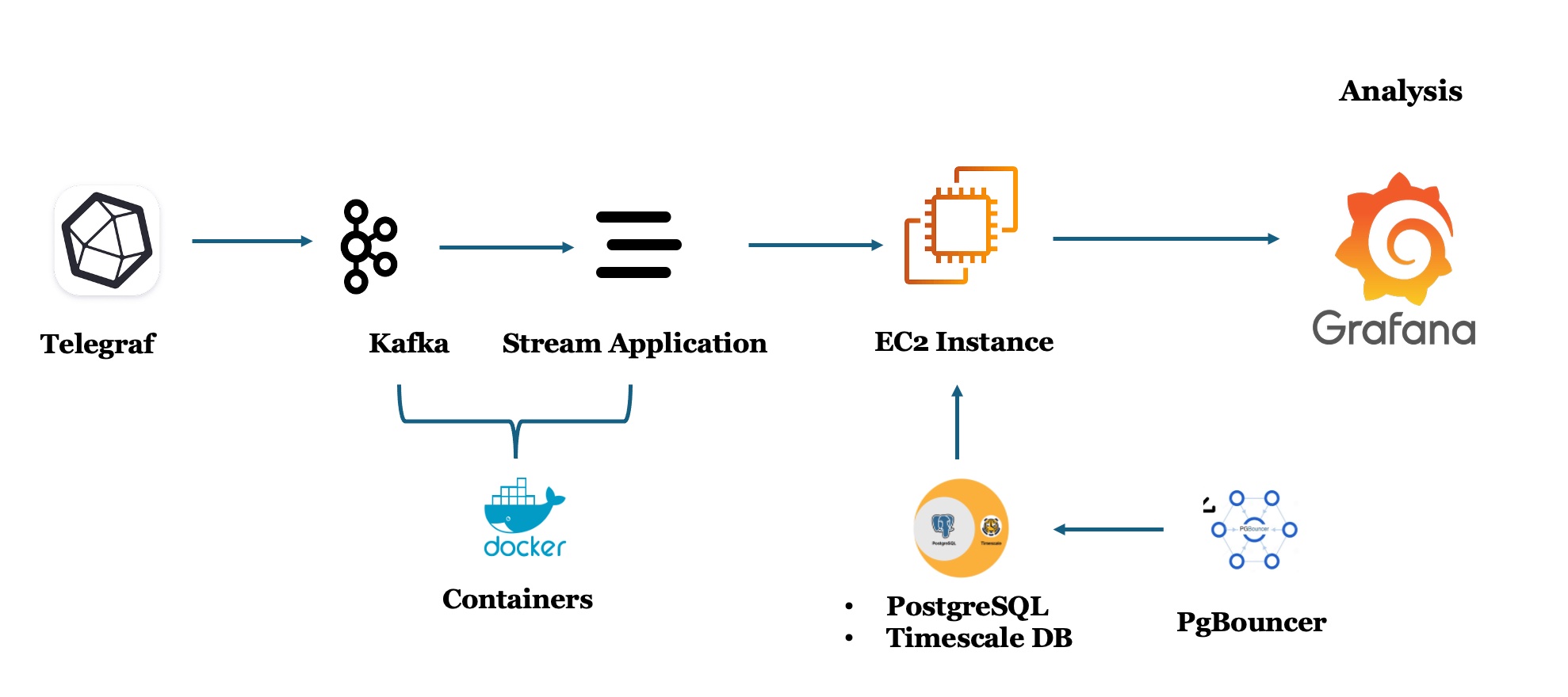
Architecture Overview

• Kafka – message broker and stream producer
• TimescaleDB (PostgreSQL) – time-series optimized storage
• PGbouncer – lightweight connection pooler
• Grafana – real-time dashboards
• AWS EC2 – cloud host for all components

Each metric (CPU, memory, network, etc.) was written to a hypertable in TimescaleDB. From there, I applied continuous aggregates and retention policies to balance performance and storage.

Continuous Aggregates for Real-Time Analytics

Raw metric tables grow fast—every second brings new readings. To prevent Grafana queries from scanning millions of rows, I created continuous aggregates that precomputed averages and maxima at short intervals.

Example for CPU metrics:

CREATE MATERIALIZED VIEW cagg_cpu_metrics_30s
    WITH (timescaledb.continuous) AS
SELECT time_bucket('30 seconds', timestamp) AS bucket,
       host,
       AVG(100 - usage_idle) AS avg_cpu_usage,
       MAX(100 - usage_idle) AS max_cpu_usage
FROM cpu_metrics
WHERE cpu = 'cpu-total'
GROUP BY bucket, host;

SELECT add_continuous_aggregate_policy('cagg_cpu_metrics_30s',
    start_offset => INTERVAL '5 minutes',
    end_offset => INTERVAL '30 seconds',
    schedule_interval => INTERVAL '30 seconds');

The same logic powered:

• Memory metrics (avg_mem_usage, max_mem_usage)
• Network metrics (avg_bytes_sent, avg_bytes_recv)
• Process metrics (avg_running, avg_idle)
• Swap metrics (avg_used_percent, avg_in, avg_out)

These policies ensured continuous background refresh, so Grafana always displayed near real-time data.

Retention Policies Keep Storage in Check

Even with continuous aggregation, hypertables would balloon over time. To keep storage costs low and maintain predictable query speed, I added retention policies that automatically drop raw metrics older than 30 days:

SELECT add_retention_policy('cpu_metrics', INTERVAL '30 days');
SELECT add_retention_policy('mem_metrics', INTERVAL '30 days');
SELECT add_retention_policy('net_metrics', INTERVAL '30 days');
SELECT add_retention_policy('process_metrics', INTERVAL '30 days');
SELECT add_retention_policy('swap_metrics', INTERVAL '30 days');

With this setup, the system kept only the most recent 30 days of raw data while aggregated views preserved long-term summaries (e.g., hourly or 12-hour averages). Query performance stayed low-latency even after weeks of streaming volume.

Connection Pooling with PGbouncer

Kafka consumers, continuous aggregate jobs, and Grafana dashboards all needed database access. Without pooling, TimescaleDB risked running out of connections. Introducing PGbouncer added a middle layer that reused sessions and smoothed throughput under high concurrency.

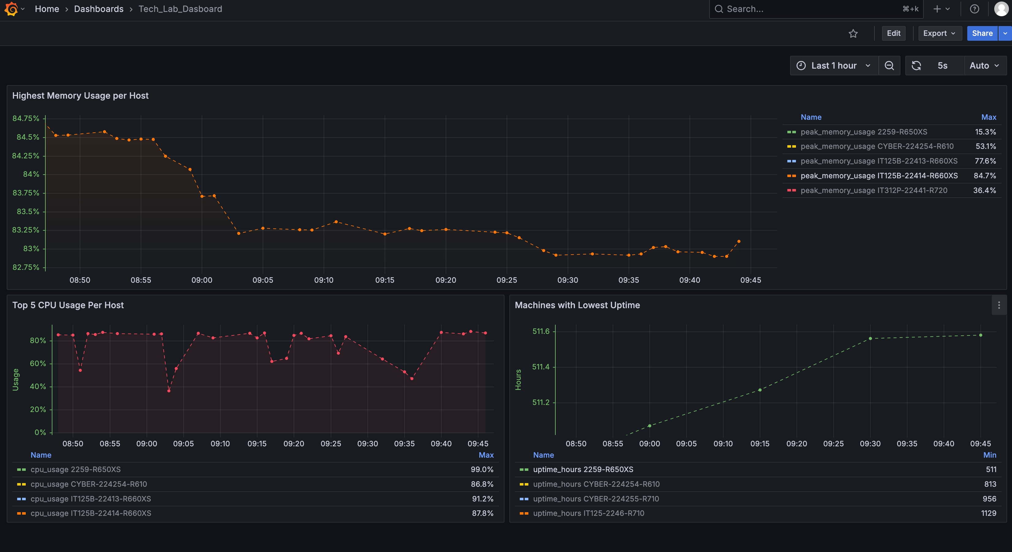
Visualization with Grafana

Grafana dashboards displayed CPU, memory, and disk usage trends, network throughput, active process counts, and overall system load. By querying continuous aggregates, panels refreshed every few seconds without noticeable delay.

Key Takeaways

• Continuous aggregates are the backbone of efficient time-series analytics.
• Retention policies prevent unbounded growth and keep performance predictable.
• Connection pooling with PGbouncer stabilizes load across multiple clients.
• Optimization is a continuous process—especially in streaming environments.

Conclusion

This project taught me how to optimize an end-to-end real-time data pipeline—from streaming ingestion to visualization—by combining data engineering, database tuning, and DevOps practices. Balancing data freshness, query latency, and storage efficiency turned a raw Kafka stream into a smooth, responsive Grafana dashboard that runs efficiently at scale.

Tags: Kafka, TimescaleDB, PostgreSQL, PGbouncer, Grafana, AWS, Real-Time Analytics